Temp Hum Prediction Model
Time-series forecasting on wireless-sensor-network data
- 3
- sensor targets
- 6×
- cross-validation folds
- WSN
- IoT time-series
- ★ 2
- stars
- Jul 2026
- last push
An end-to-end forecasting pipeline over a wireless-sensor-network dataset, predicting temperature, humidity and light from correlated environmental signals with SARIMAX and ML baselines, validated across rolling folds.
IoT Sensor Data Preprocessing, Feature Engineering, and Forecasting
This repository contains a Jupyter notebook for preprocessing IoT environmental sensor data, engineering time-series features, and benchmarking forecasting models for temperature, humidity, and light.
Notebook: preprocess.ipynb
What The Notebook Does
The notebook is an end-to-end IoT time-series pipeline. It loads MongoDB records, cleans timestamp irregularities, removes outliers, interpolates missing measurements, builds predictive features, analyzes feature importance, and evaluates both linear regression and SARIMAX forecasting models
Core stages :
- MongoDB ingestion.
- Timestamp normalization and gap repair.
- Outlier removal with z-score and IQR rules.
- Interpolation of missing numeric measurements.
- Feature engineering for temporal, rolling, lag, and cross-sensor behavior.
- Correlation and feature-importance analysis.
- Forecasting with time-series cross-validation.
- Export of plots, metrics, and Excel reports.
Data Source
The notebook expects one MongoDB document per sensor measurement with these fields
| Column | Type | Description |
|---|---|---|
timestamp |
datetime or datetime-like string | Measurement time |
light_raw |
numeric | Raw light sensor reading |
temperature_c |
numeric | Temperature in Celsius |
humidity_percent |
numeric | Relative humidity percentage |
solar_raw |
numeric | Raw solar sensor reading |
battery_v |
numeric | Sensor battery voltage |
MongoDB _id values are excluded during loading:
cursor = input.find({}, {"_id": 0})
df = pd.DataFrame(list(cursor))
Important Safety Note
One notebook cell modifies the MongoDB source collection:
input.delete_many(time_cutoff)This deletes records from MongoDB after the configured cutoff timestamp. If you are running the notebook on your own dataset, either:
- Run it against a copied collection, or
- Remove/comment out the
input.delete_many(time_cutoff)line before execution.
For reproducible research, the safest approach is to preserve the raw collection untouched and perform all deletions only inside the DataFrame.
Local Setup
1. Install Python
Use Python 3.10 or newer.
Check your version:
python --versionIf Python is not installed, download it from:
https://www.python.org/downloads/
2. Clone Or Download This Repository
If the project is hosted on GitHub:
git clone https://github.com/thonos-cpu/Temp_Hum_Prediction_Model
cd Temp_Hum_Prediction_Model
If you downloaded a ZIP file, extract it and open a terminal inside the project folder.
3. Create A Virtual Environment
On Windows PowerShell:
python -m venv .venv
.\.venv\Scripts\Activate.ps1
On macOS or Linux:
python3 -m venv .venv
source .venv/bin/activate
4. Install Required Packages
Install the libraries used by the notebook:
pip install jupyter pymongo python-dotenv matplotlib pandas numpy scipy seaborn scikit-learn statsmodels openpyxlOptional but recommended:
pip install notebook ipykernelRegister the virtual environment as a Jupyter kernel:
python -m ipykernel install --user --name iot-preprocessing --display-name "Python (IoT Preprocessing)"MongoDB Setup
Option A: Use A Local MongoDB Server
Install MongoDB Community Server from:
https://www.mongodb.com/try/download/community
Start MongoDB locally. The default host and port are usually:
host: localhost
port: 27017
Option B: Use MongoDB Atlas
If you use MongoDB Atlas, configure your connection details in the same environment file described below. You may need to adapt the URI construction cell in the notebook if your Atlas connection string uses the mongodb+srv:// format.
Environment Configuration
Create a file named credentials.env in the same folder as preprocess.ipynb.
For a local MongoDB server without authentication:
MONGO_HOST=localhost
MONGO_PORT=27017
MONGO_DB=your_database_name
MONGO_COLLECTION=your_collection_name
MONGO_USERNAME=
MONGO_PASSWORD=
For a MongoDB server with username and password:
MONGO_HOST=localhost
MONGO_PORT=27017
MONGO_DB=your_database_name
MONGO_COLLECTION=your_collection_name
MONGO_USERNAME=your_username
MONGO_PASSWORD=your_password
The notebook loads this file with:
load_dotenv("credentials.env")Preparing Your Own Dataset
To run the notebook on your own sensor data, your MongoDB collection should contain one document per measurement. A minimal example document looks like this:
{
  "timestamp": "2026-05-17T16:08:45.889Z",
  "light_raw": 42.0,
  "temperature_c": 23.4,
  "humidity_percent": 51.2,
  "solar_raw": 37.0,
  "battery_v": 2.91
}
Before running the notebook, make sure that:
timestampvalues are valid datetimes or strings Pandas can parse.- Numeric sensor fields do not contain text labels.
- All required columns exist.
- The collection contains enough chronological data for rolling windows and time-series splits.
- The records are from one consistent sensing setup or from sensors that are comparable.
The notebook assumes a sampling interval around 20 seconds. If your device samples at a different rate, update the timestamp-cleaning thresholds:
if diff < 17:
    continue
if diff > 24:
missing_times = pd.date_range(
start=cur + pd.Timedelta(seconds=20),
end=nxt - pd.Timedelta(seconds=17),
freq="20s"
)For example, if your device samples every 60 seconds, you should adjust the duplicate threshold, missing-data threshold, and interpolation frequency accordingly.
Dataset-Specific Parameters To Review
Before using the notebook with a new dataset, review these hard-coded assumptions.
Sensor Failure Cutoff
The current notebook removes data after:
2026-05-20 09:49:55.647 UTCThis was chosen for the original TelosB experiment because the sensor stopped working after battery drain. For your own data, change or remove this cutoff:
cutoff = pd.Timestamp(
    year=2026,
    month=5,
    day=20,
    hour=9,
    minute=49,
    second=55,
    microsecond=647000,
    tz="UTC"
)
Raw Light And Solar Threshold
The notebook removes readings where:
light_raw >= 150
solar_raw >= 150
This was chosen because the original dataset had an abnormal spike above 1200. For another device, inspect your sensor range before keeping this rule.
Outlier Rules
The notebook applies:
- z-score filtering with threshold
3. - IQR filtering with multiplier
2.2.
These are reasonable general-purpose filters, but they can remove valid rare events. If rare spikes matter in your domain, tune these thresholds or disable one of the filters.
Forecast Horizon
The linear regression forecasting section uses:
horizon = 100Because the cleaned data is approximately 20-second sampled, this predicts roughly:
100 * 20 seconds = 2000 seconds = about 33 minutes
If your sampling interval changes, the real-world prediction horizon changes too.
Running The Notebook
Start Jupyter:
jupyter notebookThen open:
preprocess.ipynb
Select the kernel:
Python (IoT Preprocessing)
Run the notebook from top to bottom.
In Jupyter Notebook, use:
Kernel > Restart & Run All
In JupyterLab, use:
Run > Restart Kernel and Run All Cells
Generated Files
The notebook may generate:
| File | Purpose |
|---|---|
pipeline_results.pkl |
Cached feature matrices, correlations, and feature scores |
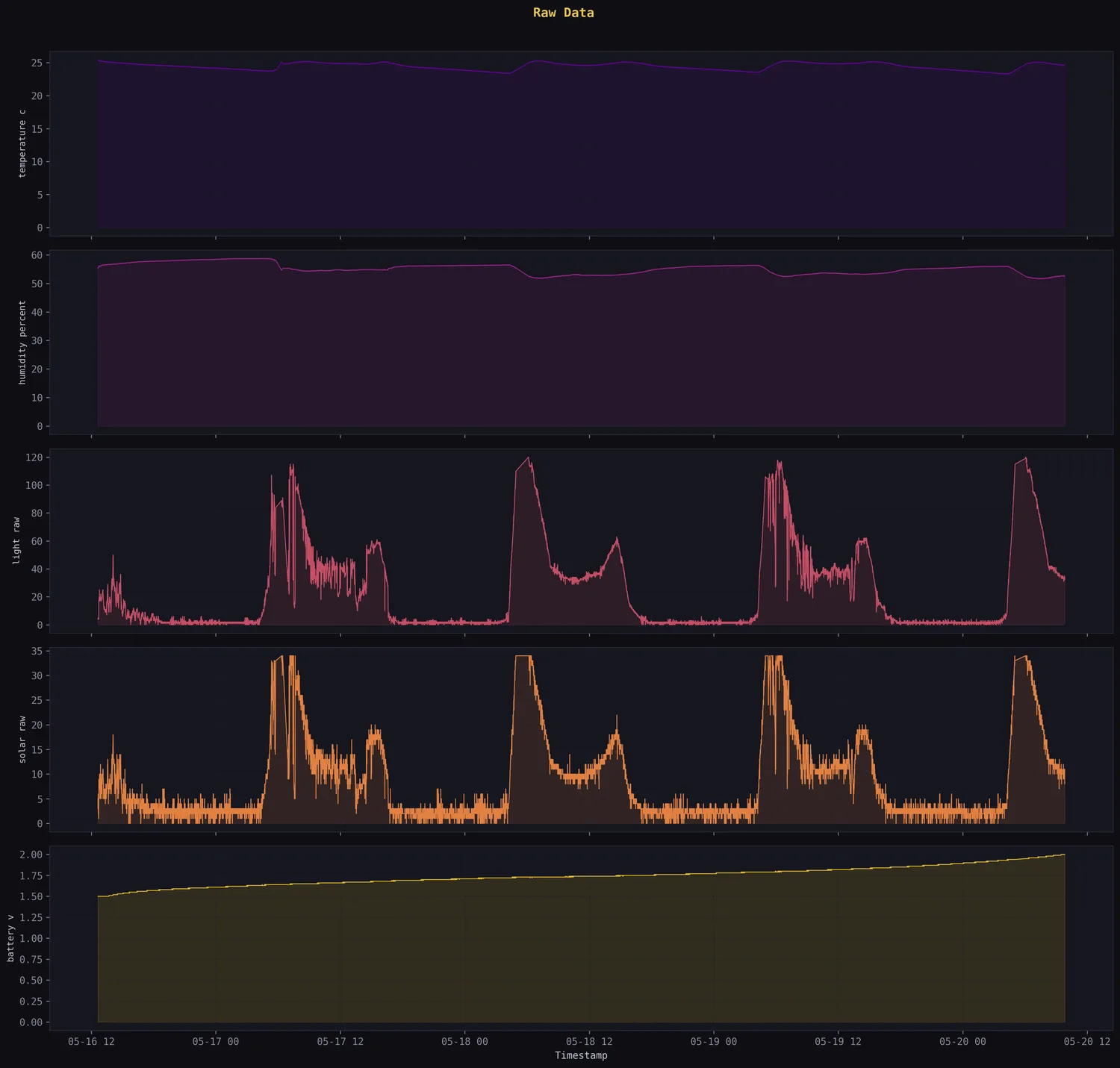
01_raw_timeseries.png |
Raw sensor time-series plot |
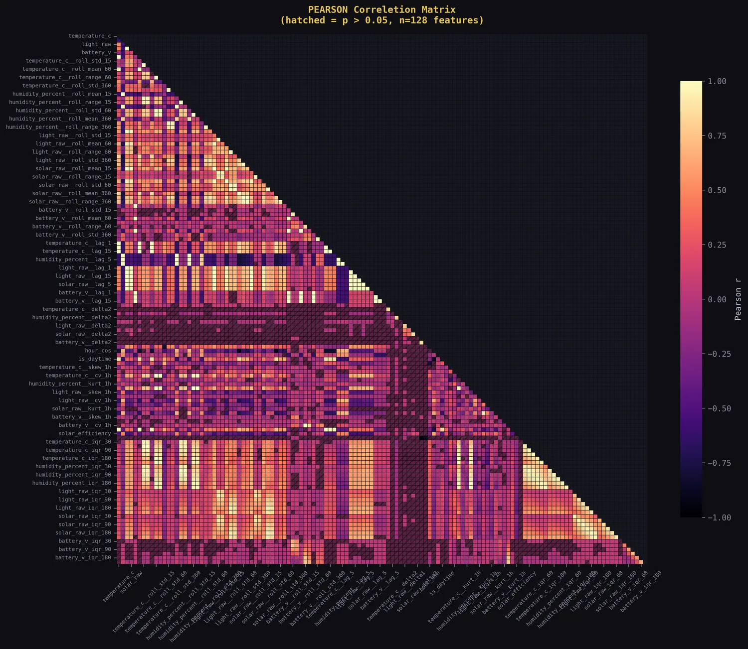
02_corr_heatmap_pearson.png |
Pearson feature-correlation heatmap |
02_corr_heatmap_spearman.png |
Spearman feature-correlation heatmap |
03_sensor_corr_heatmap.png |
Raw sensor correlation heatmap |
05_diurnal_boxplots.png |
Hourly sensor distribution plots |
target_*_fold_*_pred.png |
Fold-level regression prediction plots |
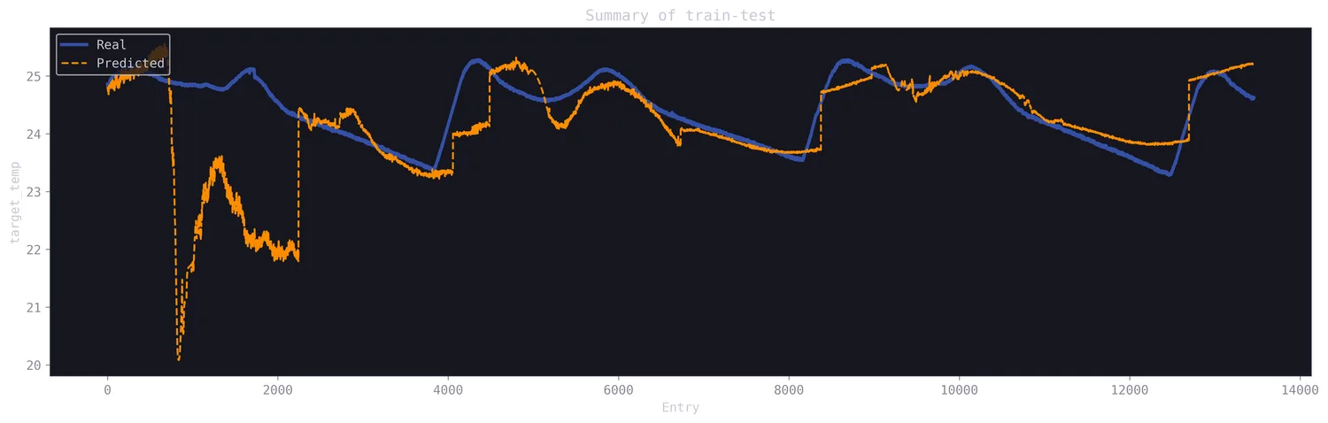
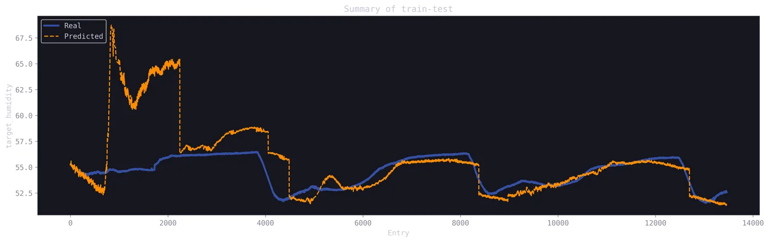
target_*_predicted_summary.png |
Full prediction summaries |
time_series_metrics.xlsx |
Linear regression metrics |
sarimax.xlsx |
SARIMAX metrics |
Feature Engineering Details
The notebook builds a compact but rich feature space:
| Feature family | Examples |
|---|---|
| Rolling windows | mean, standard deviation, range over 15, 60, and 360 minutes |
| Lag features | previous values at lag 1, 5, and 15 |
| Delta features | first-order and second-order differences |
| Diurnal features | hour_sin, hour_cos, day_of_week, is_daytime, hour_bin |
| Statistical features | rolling skewness, kurtosis, coefficient of variation |
| Cross-sensor features | heat index proxy, solar efficiency, battery drain rate |
| IQR features | rolling interquartile range across multiple windows |
Modeling Approach
Linear Regression
The notebook predicts future temperature_c, humidity_percent, and light_raw values with multi-output linear regression. Targets are shifted by horizon = 100, and evaluation uses TimeSeriesSplit(n_splits=6).
Reported metrics include MAE, MSE, RMSE, train/test R2, median absolute error, explained variance, max error, residual mean, and overfitting gap.
SARIMAX
The notebook also fits SARIMAX models for the same three sensor targets using exogenous variables such as solar_raw, battery_v, cyclical time features, and lagged sensor values.
Configuration:
order=(2, 0, 1)
TimeSeriesSplit(n_splits=5, test_size=300)
Reported metrics: MAE, MSE, RMSE, and R2.
Recommended Workflow For New Experiments
For a clean experiment on a new dataset:
- Import your raw measurements into a MongoDB collection.
- Back up the raw collection.
- Create
credentials.env. - Open the notebook.
- Remove or modify the original experiment cutoff.
- Adjust sampling-interval thresholds if your device does not sample every 20 seconds.
- Inspect raw plots before keeping the outlier thresholds.
- Run preprocessing cells.
- Validate the cleaned signal plots.
- Run feature engineering and correlation analysis.
- Review the selected features and correlation heatmaps.
- Run forecasting models.
- Compare regression and SARIMAX metrics.
- Use exported plots and Excel files for reporting.
Reproducibility Notes
The notebook uses deterministic settings where applicable, including:
random_state=42for mutual information and random forest feature scoring.
Some results may still vary across library versions, especially SARIMAX optimization results and floating-point numerical routines. For publishable experiments, record your package versions:
pip freeze > requirements-lock.txtTroubleshooting
ModuleNotFoundError
Install the missing package:
pip install <package-name>For the notebook as written, the most important packages are:
pymongo
python-dotenv
pandas
numpy
matplotlib
scipy
seaborn
scikit-learn
statsmodels
openpyxl
MongoDB Connection Fails
Check that:
- MongoDB is running.
MONGO_HOSTandMONGO_PORTare correct.- The database name exists.
- The collection name exists.
- Username and password are correct if authentication is enabled.
- Your IP address is allowed if using MongoDB Atlas.
Empty DataFrame
If df has zero rows:
- Confirm the collection contains documents.
- Confirm the environment variables point to the right database and collection.
- Confirm the notebook connects to the expected MongoDB instance.
Timestamp Errors
If timestamp parsing fails, normalize your timestamps before import or adjust:
pd.to_datetime(df["timestamp"], utc=True)Too Many Rows Dropped
If the cleaned dataset becomes too small, review:
- The sensor failure cutoff.
- The
light_raw < 150andsolar_raw < 150filters. - The z-score threshold.
- The IQR multiplier.
- The rolling-window sizes.
- The forecast horizon.
Suggested Repository Structure
A clean GitHub version of this project could use:
.
├── README.md
├── preprocess.ipynb
├── requirements.txt
├── .gitignore
└── examples/
    └── sample_document.json
Do not commit real credentials. Add this to .gitignore:
credentials.env
*.pkl
*.xlsx
*.png
.venv/
__pycache__/
Project Summary
This notebook turns raw MongoDB IoT measurements into cleaned signals, engineered features, diagnostic plots, and forecasting benchmarks for environmental sensor data.